
**This article is not finished, though it’s in good enough shape to get my ideas across. There may be inaccuracies, misspellings, or grammar errors. There is also much more work to do. This site is a living document. I am an amateur. This is basically just my opinion. I am only hoping to inspire others more capable than myself.
**Also be sure to check out the calculator. I think it does a pretty good job of explaining this stuff in a visual way. https://theuniverseisnotexpanding.com/calculator/
The proposed cosmological model can be summarized with the following postulates.
- All objects are embedded within larger-scale objects.
- Mass density is inversely proportional to any given radius >1Mpc.
- Gravitational binding occurs across all scales.
- There is a minimum threshold for gravitational acceleration g.
- H0 is gravitational redshift.
- The CMBR is caused by Hawking radiation at the observable radius.
- The observable universe can be modeled with the interior solution to the Schwarzschild metric.
Introduction
At its core, cosmology seeks to accurately describe the distribution of matter and energy in the universe. Typically, this is accomplished by satisfying the Einstein Field Equations, which in turn describe the overall geometry of the universe.
For nearly a full century now cosmologists have used the FLRW metric for the largest scales. It’s a simple and intuitive approach that explains the Hubble redshift. The FLRW metric has three possible options – expansion, collapse, or in-between. Expansion is not an inherent feature or direct prediction of general relativity. The expanding solution comes specifically from the assumptions and boundary conditions chosen in the formulation of the FLRW metric. [1,2]
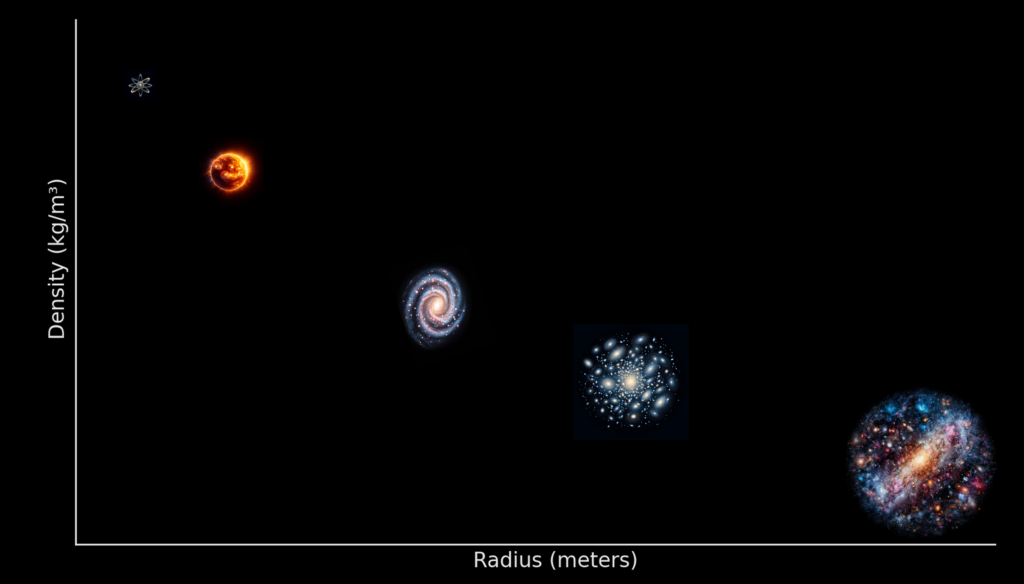
However, in spite of what cosmologists claim, our Universe is not homogeneous. The Universe is not even nearly homogenous. Mass density varies across all scales. Stars, galaxies, clusters of galaxies, super clusters, filaments, veins, walls, and the observable universe all have a different mass density ρ.
The hierarchical structure of the cosmos follows an inverse relationship, as all objects are embedded within other objects. The most significant difference with this distribution is that it predicts a gravitational redshift that is directly proportional to the distance of light travel (more on this in a moment).
Historical Context
The modern interpretation of the Schwarzschild metric focuses on the fact that it predicts black holes and even horizons. But Schwarzschild’s original 1916 solution does not mention either of the two. Instead, the paper lays out the geometrical structure of spacetime surrounding a non-rotating, spherically symmetric mass.
Schwarzschild’s original 1916 solution was groundbreaking and intuitive, but Einstein and others in the physics community met his solution with skepticism and confusion, failing to grasp its full implications. The Schwarzschild metric eventually played a crucial role in establishing the fundamental principles of general relativity and advancing the scientific understanding of gravitational physics during that era., but it has never been considered as a cosmological model. [3,4]
On the other hand, the FLRW metric, independently derived by Alexander Friedmann, Georges Lemaître, Howard P. Robertson, and Arthur Geoffrey Walker during the 1920s and 1930s, is a solution to Einstein’s field equations that describes a homogeneous and isotropic expanding (or contracting) universe. It has been the cornerstone of modern cosmology because of its adherence to the cosmological principle, which posits that the universe is homogeneous and isotropic on large scales.
Despite its success, the Lambda-CDM model, under the umbrella of the FLRW metric, still grapples with inherent limitations and unsatisfactory explanations, relying on unobservable constructs such as dark matter, dark energy, and inflation.
- The FLRW metric does not predict an expanding metric.
- The expansion cannot be accounted for using general relativity.
- The rate of expansion increases over time.
- The rate of expansion was highest during the earliest part of the universe.
- Gravity is a phenomenon that results in attraction.
Theoretical Framework
“The misconception which has haunted philosophic literature throughout the centuries is the notion of ‘independent existence. ‘ There is no such mode of existence; every entity is to be understood in terms of the way it is interwoven with the rest of the universe.”
Alfred N. Whitehead [5]
The quote above highlights the complications involved in creating an accurate cosmological model. The average galaxy is several orders of magnitude more dense than the observable universe. However, galaxies are typically part of a galaxy cluster, and galaxy clusters reside within superclusters, which reside within larger-scaled structures. All objects are embedded within other objects.
The Schwarzschild metric was chosen to represent this framework because it best represents what one is able to predict when making a cosmological observations. The observable universe is literally a non-rotating, spherically symmetric, massive object. The interior solution was chosen to represent the perspective of being inside the observable universe.
Gravitational boundaries are fundamentally arbitrary. There is no clear boundary between one star and another. Atoms blend together to form stars. Trillions of stars all blend together to form galaxies, it all blends together to create the universe. However, the observable universe is a definitive boundary, albeit a fictious boundary.
In the context of general relativity, the concept of a gravitational “boundary” refers to something like an event horizon. On the other hand, the surfaces of stars, planets, and galaxies are determined by a complex interplay of various forces (gravitational, electromagnetic, nuclear, etc.), matter distributions, and conditions. These “boundaries” are more fluid and are not defined in the same fundamental way as something like an event horizon or the observable radius.
Mathematical Formulation
The proposed hierarchical structure can be formulated with a uniform gravitational acceleration g. The idea is not to refer to Newtonian concepts within a geometric framework, but to utilize the density distribution that comes along with a uniform g. You can call it the Newtonian cosmological constant if you’d prefer that. I call it gravitational acceleration. Regardless, the phenomenon occurs because there is a minimum density on cosmological scales, resulting in a minimum g. The following parameters are based on the value of H0.
g – Gravitational acceleration (also g) ~ 3.5× 10⁻¹⁰ m/s2
G – Gravitational constant, 6.674 × 10⁻¹¹ m3 kg−1 s−2
ρ – Mass density – 9.7 × 10⁻²⁷ kg/m3
r – Distance of light travel; radial coordinates from the source to the observer
rs– The Schwarzschild radius; observable radius ~ 1.2839 × 1026 m/s
c – The speed of light, 299,792,458 m/s
H0– Hubble constant, ~72 km/s Mpc
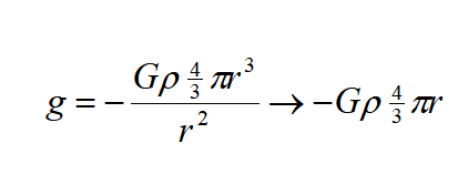
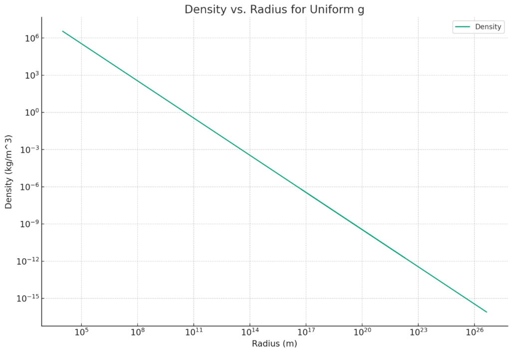
Here, the relation of g to the density distribution for the volume of space with radius r.
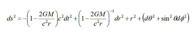
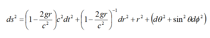
The line element for the Schwarzschild solution can be written as:
To derive an interior solution, we convert mass to density and the inverse relationship.
We can further simplify using g, which automatically includes the inverse mass density relationship.
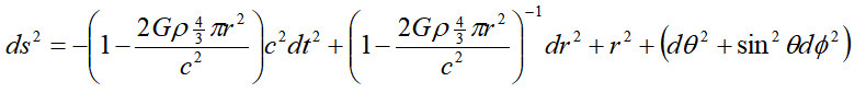
The equation for the interior Schwarzschild solution is given by the line element:
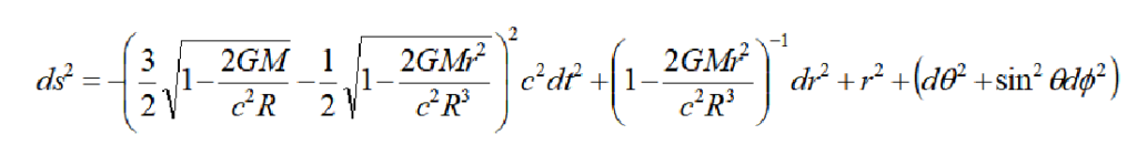
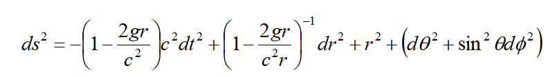
Again, we change the homogeneous distribution to the variable density using the Newtonian approximation for gravitational acceleration g.
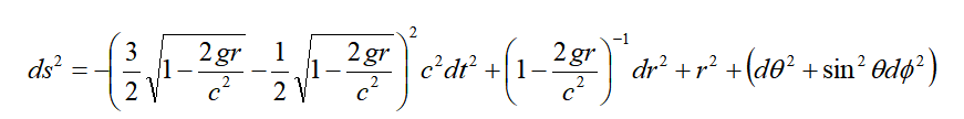
Which reduces to the line element for the exterior solution.
Smoothly matching f(r) to the Schwarzschild potential at the boundary r = R provides continuity between the interior and exterior regions (observable radius for cosmology). Varying the density profile ρ(r) allows for modeling different spherically symmetric mass distributions within this consistent metric framework.
Specifying a radial density profile ρ(r) allows flexibility in modeling the object’s interior composition. The interior metric form with f(r) perturbing the spatial part is justified based on typical forms of GR solutions. Relating f(r) to the enclosed mass M(r) through the -2GM(r)/rc2 potential aligns with gravitational time dilation effects described by GR.
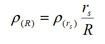
For starlight, this framework predicts a gravitational redshift that is directly proportional to the distance of light travel, r, assuming the observer resides within a region of the universe with no local gravitational effects. For cosmological distances, light must transverse many different scales. The journey begins at the surface of star. Here, the density of mass is the highest the light will ever encounter (for light we observe from earth). From the moment it is released it begins to climb uphill. As the light transverses outward from the source, it encompasses a larger and larger volume of space. The density of this volume decreases until it reaches the minimum density on the scale of the observable radius, while the gravitational potential increases and g reaches maximum uniformity.
Working backwards from the Hubble parameter, now being interpreted as gravitational redshift, we obtain the following the density profile for the observable universe (4163 Mpc), when H0≈72,000 m/s/Mpc, the observable radius occurs around 1.283× 1026 meters, with the mass density around 9.7× 10⁻²⁷ kg/m3.
This distribution profile reflects the hierarchical structure of our universe. On smaller scales, we find denser structures such as stars and galaxies. As we move to larger scales, the average density decreases, with galaxy clusters, superclusters, and large-scale structures like cosmic filaments and walls having lower average densities, and the observable radius possessing the lowest density.
Dark Energy
Over the past couple of decades, observations of distant Type 1a supernovae have been found to be fainter than expected. “Dark Energy” was coined as the source of the accelerating expansion, but the phenomenon is really just an adjustment to the cosmological constant. Even still the underlying physics behind expansion and acceleration remain a mystery. [6,7]
The difference between the three models is subtle until the z≈2 region, but the difference would be very difficult to detect from real world observations from any distance less than z≈4. It might be possible to decipher the data if determinations of the luminosity distance function could be trusted from sources beyond 4000 Mpc, or using very large data sets. Regardless, DE is not necessary within SIC.
Dark Matter
Dark matter is a proposed type of matter used to explain the unexpected rotation curves of galaxies, which can’t be accounted for by the amount visible matter. It supposedly doesn’t emit, absorb, or reflect any electromagnetic radiation, making it detectable only through its gravitational effects. Cosmological models have very little to do with the dynamics of galaxies. However, this model does provide an approximation for the mass and density of objects based on their radius, which could provide insights into the missing mass anomaly. [8]
MOND, or Modified Newtonian Dynamics, modifies Newton’s second law at very low accelerations, typical of galactic scales, where the gravitational acceleration a0 is much smaller than a certain threshold a0.
The commonly accepted value of a0 is approximately 1.2×10⁻¹⁰m/s2, indicating the acceleration below which the modification to Newton’s laws becomes significant and above which classical Newtonian dynamics is recovered. [9]
The theoretical underpinnings of the MOND acceleration threshold, a0 and its specific value remain subjects of ongoing research and debate. While MOND phenomenologically succeeds in explaining galaxy rotation curves and the Tully-Fisher relation without invoking dark matter, the fundamental origin of a0 is not derived from first principles within the original MOND framework. [10]
Within the SIC model, the minimum threshold for gravitational acceleration comes from total mass of the observable universe.
Cosmic Microwave Background Radiation
Perhaps the most discussed feature of the Schwarzschild solutions is that they predict the the potential existence of black hole singularities. The famous equation to find the Schwarzschild radius for an object with mass M is as follows:
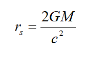
Typically rs is much smaller than r. For example, a black hole with a mass equaling 1M☉ would have a radius around 3 kilometers. The
Starlight originating from the beyond the observable radius would be redshifted to the point of unobservability. However, the temperature of Hawking radiation is given by:

For the observable universe, the predicted temperature is incredibly insignificant 1 × 10⁻³⁰ Kelvin. However, this radiation is created by quantum mechanical effects, as opposed to being emitted from a star, meaning it would begin its journey at the absolute minimum gravitational potential. From our perspective, the CMBR radiation is just beyond the observable radius. In this case, the factor of change due to gravity would be the absolute upper limit. [11,12]
One potential option to find the limits on relativistic effects could be to utilize the Planck length and the Schwarzschild radius. To find the final observed wavelength λ based on the factor of change from the gravitational effects of the observable universe:
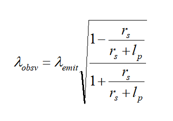
Using the parameters from above, the maximum factor of change for the wavelength of light due to blue shifting is 1.839× 10⁻³¹ .
Using Wien’s displacement law, the predicted peak temperature of the final observed, blue shifted, Hawking radiation is 6.1Kelvin.
Being off by a factor of 2 could mean any number of things. The observable radius, density, g, and the upper limit to the factor of change are all up for grabs, but they’re most likely off by a little.
If the above methods are accurate, then it should fairly easy to fine-tune the parameters based the CMBR temperature of 2.7Kelvin. However, doing so reduces the Hubble parameter to 30 km/s Mpc, well below the surveyed value. The problem is almost certainly in my method to formulate an upper limit the factor of change.
My Twitter- Hillbilly (@BestCosmologist) / X (twitter.com)
My YT Channel – https://www.youtube.com/@BestCosmologist
Click here to email meReferences
- Wikipedia contributors. (n.d.). Friedmann–Lemaître–Robertson–Walker metric. In Wikipedia, The Free Encyclopedia. Retrieved from https://en.wikipedia.org/wiki/Friedmann–Lemaître–Robertson–Walker_metric
- LibreTexts. (2021, August 16). 7.2: The Friedmann-Lemaitre-Robertson-Walker Metric. In Physics LibreTexts. Retrieved from https://phys.libretexts.org/Bookshelves/Relativity/Book%3A_Introduction_to_General_Relativity_(Crowell)/07%3A_Cosmology/7.02%3A_The_Friedmann-Lemaitre-Robertson-Walker_Metric
- Wikipedia contributors. (n.d.). Schwarzschild metric. In Wikipedia, The Free Encyclopedia. Retrieved from https://en.wikipedia.org/wiki/Schwarzschild_metric
- O’Connor, J. J., & Robertson, E. F. (n.d.). Karl Schwarzschild (1873 – 1916). MacTutor History of Mathematics Archive. Retrieved from https://mathshistory.st-andrews.ac.uk/Biographies/Schwarzschild/
- Whitehead, A. N. (1925). Science and the modern world. The Free Press. p. 64.
- Ray, J. (2021, November). Type Ia supernovae: Inside the universe’s biggest blasts. Astronomy. Retrieved from https://www.astronomy.com/news/2021/11/type-ia-supernovae-inside-the-universes-biggest-blasts.
- Wikipedia contributors. (n.d.). Type Ia supernova. In Wikipedia, The Free Encyclopedia. Retrieved https://en.wikipedia.org/wiki/Type_Ia_supernova.
- Rubin, V. C., Ford, W. K., Jr., & Thonnard, N. (1978). Extended rotation curves of high-luminosity spiral galaxies. IV – Systematic dynamical properties, Sa through Sc. The Astrophysical Journal, 225, L107-L111.
- Scarpa, R. (2006). Modified Newtonian Dynamics, an Introductory Review. arXiv preprint arXiv:astro-ph/0601478. Retrieved from https://ar5iv.org/abs/astro-ph/0601478
- Milgrom, M. (2001). MOND—a pedagogical review. arXiv preprint arXiv:astro-ph/0112069. Retrieved from https://ar5iv.org/abs/astro-ph/0112069
- Penzias, A. A., & Wilson, R. W. (1965). A measurement of excess antenna temperature at 4080 Mc/s. Astrophysical Journal, 142, 419-421.
- Hawking, S. W. (1974). Black hole explosions? Nature, 248(5443), 30-31.